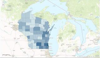
GIS 1, Lab 4
Goal and Background:The goal of Lab 4 was to assemble attribute and spatial query expressions to acquire information from the data.
Methods:
The first step to Lab 4 was setting my geoprocessing workspace and scratch space to my Lab 4 folder in ArcMap. I added the counties data from the U.S. geodatabase in order to write queries for the first three criteria. The first question wanted to return counties with a population between 3000 and 4000 in 2010 and counties with a population density of at least 1000 persons per square mile in 2010. I wrote out the query in the select by attributes tab to say SELECT * FROM counties WHERE: (POP2010 > 3000 AND POP2010 < 4000) OR (POP10_SQMI >= 1000). I exported the selected attributes to my Lab 4 folder and displayed the data onto the counties layer. In layer view, I created a cartographically pleasing map of the counties that meet the criteria to include a scale bar, north arrow, legend, title, and a description on the selected features (Figure 1).
The second question asked to return counties in Wisconsin, Texas, New York, Minnesota, and California where the male population is greater than the female population and the population of seniors is over 6500.After setting up a new map of the counties, I wrote out the query in the select by attributes tab to say SELECT * FROM counties WHERE: (STATE_NAME IN ('Wisconsin', 'Texas', 'New York', 'Minnesota', 'California') AND MALES > FEMALES) AND (STATE_NAME IN ('Wisconsin', 'Texas', 'New York', 'Minnesota', 'California') AND AGE_65_UP > 6500). I exported the selected counties to my Lab 4 folder and displayed it as its own layer on top of the counties layer. Switching from data view to layer view, I created a map with the same qualities as the previous one (Figure 2).
The next criteria asked to return counties is Washington, Maryland, Illinois, District of Columbia, Nebraska, and Michigan where there are more than 30,000 housing units available in addition to the previous query. I opened the select by attributes tabs and assembled the query to read SELECT * FROM counties WHERE: (STATE_NAME IN ('Wisconsin', 'Texas', 'New York', 'Minnesota', 'California') AND MALES > FEMALES) AND "AGE_65_UP" > 6500) OR (STATE_NAME IN ('Washington', 'Maryland', 'Illinois', 'Nebraska', 'District of Columbia', 'Michigan') AND HOUSEHOLDS > 30000). Once again, I exported the selected features to my Lab 4 folder, displayed the new layer onto the map, and created a cartographically pleasing map of the counties that meet the criteria in layer view (Figure 3).
For the next part of the lab, I downloaded the Wisconsin data into my Lab 4 folder where I unzipped the data. In ArcMap, I added the Wisconsin counties, cities, and lakes data to the data frame in a new blank map. My next task was to return cities with a 2007 population between 15,000 and 20,000, with an area of at least 5 square miles, the female population is greater than the male population and are within two mile of a lake. This called for an attribute query and a spatial query. First, I opened the select by attributes tab wrote, SELECT * FROM cities WHERE: "POP2007" >= 15000 AND "POP2007" >= 20000 AND ("AREALAND" >= 5) AND ("FEMALES" > "MALES"). I applied the query and then opened the select by location tab. I specified the selection method to select from the currently selected features, target layer to be WI_cities, source layer to be lakes, and to be a distance of 2 miles from the source layer. The selected cities meeting the criteria were exported to my Lab 4 folder and displayed onto the map. I created a map of the new layer along with the roads data with the same qualities and features of the previous maps (Figure 4).
The final task wanted to know the total length in miles of thirteen rivers: Chippewa R, Eau Claire R, Embarrass R, Fisher R, Hunting R, Kinnickinnic R, Maunesha R, Milwaukee R, Moose R, Namekagon R, Pelican R, Platte R, and Potato R. First, I set up a new map with the Wisconsin counties data. In the River_ data's attribute table, I created a new field called LENGTH and calculated the geometry length for the records. I then opened the select by attributes tab assembled a query to read SELECT * FROM Rivers_ WHERE: "PNAME" IN ('Chippewa' R, 'Eau Claire R', 'Embarrass R', 'Fisher R', 'Hunting R', 'Kinnickinnic R', 'Maunesha R', 'Milwaukee R', 'Moose R', 'Namekagon R', 'Pelican R', 'Platte R', and 'Potato R'). The query selected these rivers. In the River_ data's attribute table, I viewed the statistics for LENGTH to find out the selected rivers' total length. Lastly, I exported the selected features to my Lab 4 folder, displayed it to the Wisconsin counties layer, and added the roads data and lakes data to the data frame. In layer view, I created final map of the selected features like the previous maps (Figure 5).
Results:
The following maps are the result of the previous queries in their respective order.
Figure 1
Figure 2
Figure 3
Figure 4
Figure 5
Sources:
USA data (2016) [downloaded] Price, Maribeth H. [March 29, 2017].
Wisconsin data (2011) [downloaded] ESRI. [March 30, 2017].
Wisconsin Lakes (2012) [downloaded] Wilson, Cyril. [March 30, 2017].


